Tutorial

Organizing the data

Your image(s) just need to be stored in a single folder. The Parent Folder name does not matter.

The Prediction

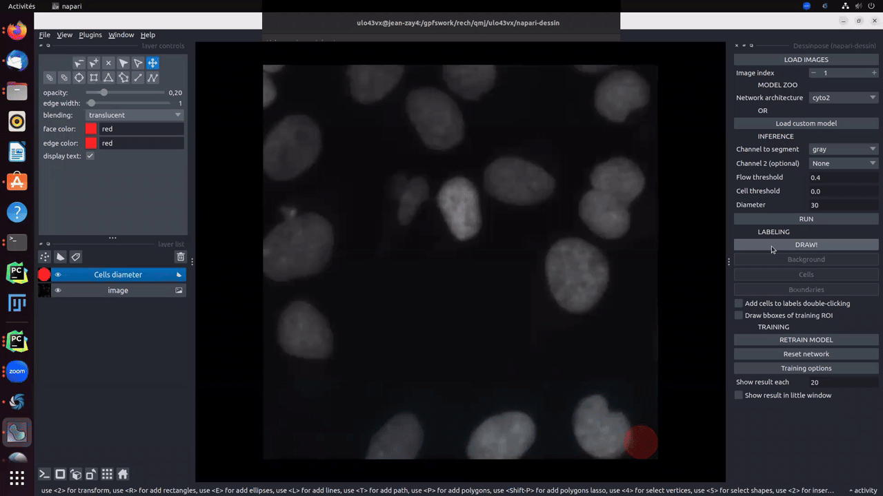
Data loading

A dedicated button called LOAD IMAGES loads the folder and displays the first image.

Switching from an image to another

You can switch to the next image clicking on →, or to the previous one clicking on ←. Also, a text field with arrows displaying the image index enables to switch from an image to an other. Switching from an image to another automatically saves the labels if they exist, and reloads them.

Choosing a model

All Omnipose models are available and can be used for inference and transfer learning:

• bact_phase_omni

• bact_fluor_omni

• cyto2_omni

• worm_omni

• plant_omni

The description of the models is available in Omnipose’s paper. You can also load a custom CellPose or Omipose model, using Load custom model button.

The Annotation

How to label

First way (recommended)

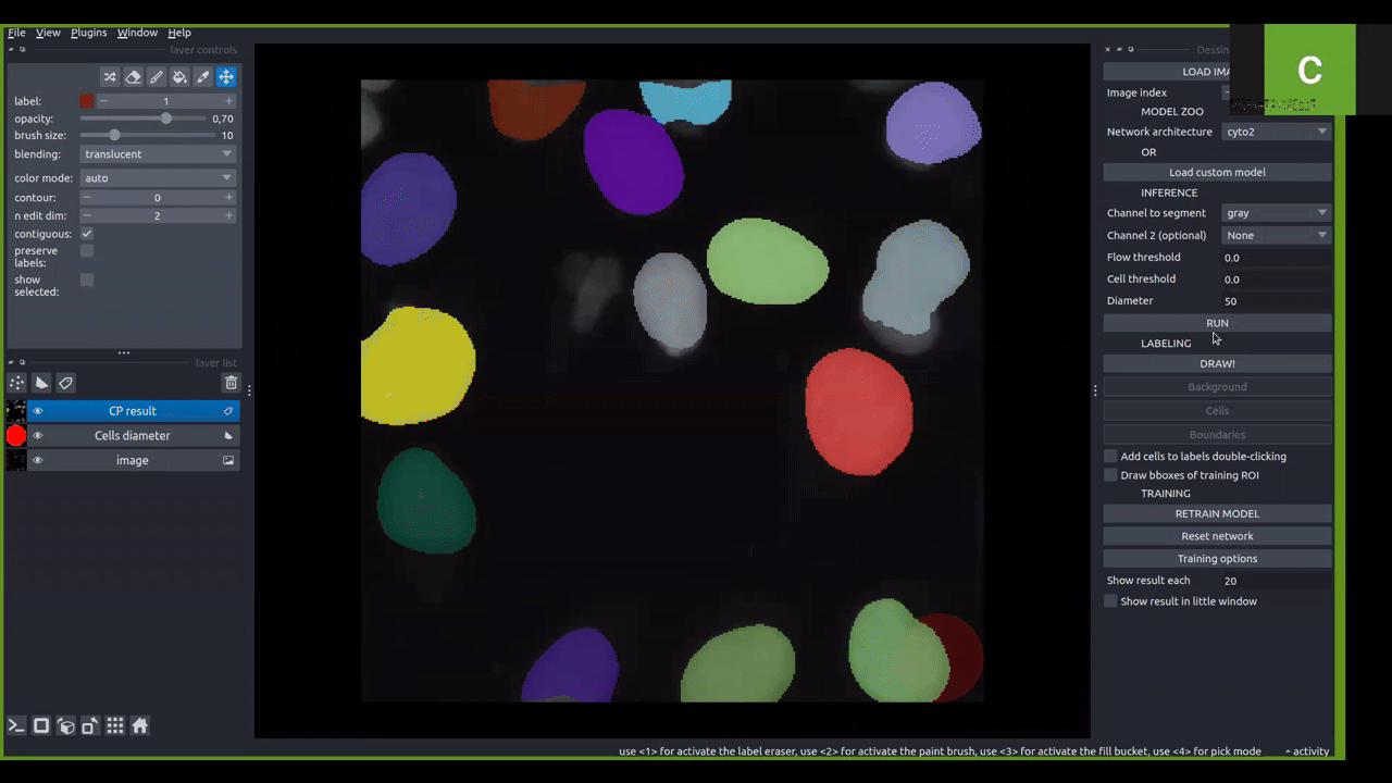
Clicking on Draw! button will create two different layers. One for cells (in blue) and background (in brown) labels, and one for the boundaries (in red). To start drawing, you must click on cells, background or boundaries depending on what the you want to draw. Size auto-adjusts as a function of the drawn item. Boundaries are thin and the brush size should not be changed. For cells and background, brush size can be changed using ↑ and ↓.

Obviously, as explained in the paper, you are not obliged to fully annotate the objects. A cell can be partially labelled. Moreover, the boundaries used for the computation of the distance map will be the combination of drawn boundaries and the intersection of cells labels and background labels. The Gif below, shows an example of partial labelling:

TRICK: When you are in drawing mode, you can drag/pan, holding space button. Hence, you are not obliged to deactivate drawing mode.

IMPORTANT: All the annotated images of your folder will be used for training. Hence, if there are some images that you do not want to use for training and that you have already labelled, manually remove their labels from the dedicated folder.

If you draw an entire cell, you can directly add its edges by right-double-clicking on the cell.

Moreover, if pretrained model gives good results on some cells, an option called add cells to labels double-clicking makes you earn time to directly add cells from the inference result to the groundtruth.

Second way

Another training approach involves reducing the annotations to bounding boxes. In this method, after the initial prediction, the user manually draws bounding boxes that encompass the areas where corrections or adjustments to the segmentation are needed. The final ground truth is then formed by combining the predictions of the pretrained model with the regions of interest (ROIs) modified by the user. This approach does not constitute partial annotation training, as the bounding boxes are required to be fully labeled within. Despite this requirement, it offers the advantage of working with smaller areas, resulting in time savings.

Note: You can see that undesired cells were removed by mouse-wheel-clicking on them.

The Training

Setting the parameters

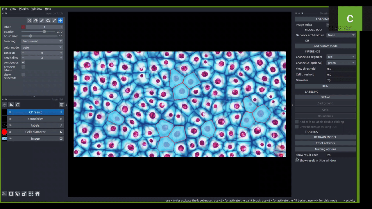
The model and the channels which are going to be used for training are the one defined in the main interface. To train from scratch, one must choose None value for the weights. Once a training is launched, the value will automatically be turned into custom model whatever the initial model.

An additional dialog window shows the other parameters the user can modify to train (from scratch) or retrain a model. The list of parameters is:

• Learning rate

• Weight decay

• Epochs number

• Use SGD: whether you want to use the SGD instead of RAdam.

Visualisation of training model’s learning

There are two different option to interactively visualize the progress of the training on the current image. The default option is the inference on the whole image each N iterations defined in the interface by the user. We do not recommend it for big images, as it will slow down the training significantly.

The second option is the visualization in a tiny window at each iteration. The window can be dragged and resized at any time.

In all cases, the training loss function is displayed in real time in the lower right-hand corner of the window.

If you want to add labels on the fly during training, you have to stop training and resume it so they are taken into account.

The gif below illustrates both ways to visualize the training progress. The training has been processed from scratch.

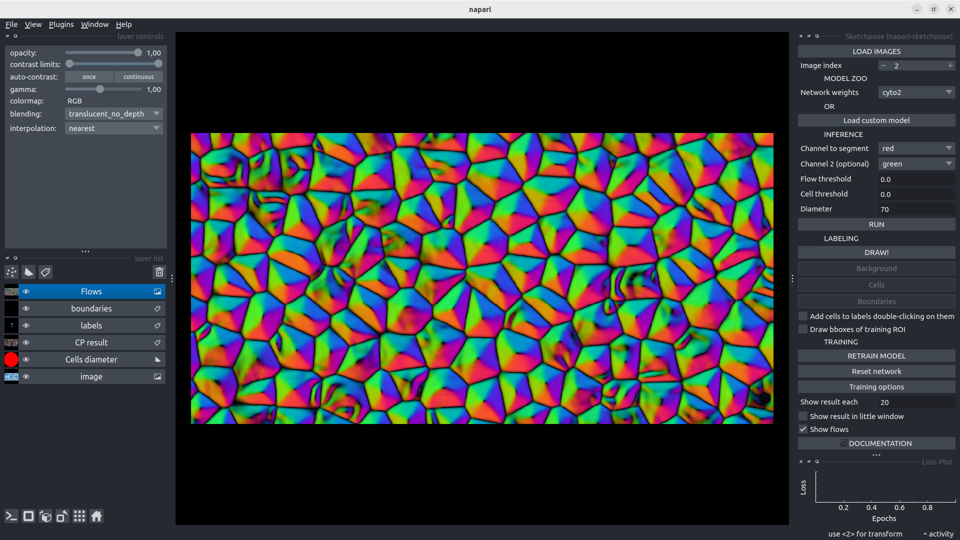
Visualisation of the flows

As in the original Cellpose/Omnipose interface, it is possible to visualize the flow for any inference (using Show flows tick case), hence while showing the training result either in the little window or in the whole image. This is a quite interesting additional information to understand in which parts of the image, the CNN does not succeed in producing accurate flows. It can guide the user through a more selective and efficient way to label the data.